
Quantum XL has been enhanced to support a number of new features. The most significant new feature is the ability for any cell to be an input and any cell to be an output. This allows existing spreadsheet models to be turned into Monte Carlo simulations very quickly and easily.
Below is a simple financial model in Microsoft Excel. The goal of this model is to predict the profit from the sales of a new product. The model has certain assumptions (called inputs) which are used to calculate various metrics (called outputs). In this model, the inputs are the competitor’s sales price for a competing product, our sales price, the market size, and the manufacturing cost.
The outputs are the Percent Market Share, which depends on our sales price and our competitor’s sales price; the Total Sales, which depends on the market size, market share, and our sales price; and finally, the Total Profit, which depends on the market size, percent market share, our sales price, and the manufacturing cost.
Download Workbook with example Model

A common activity with this approach is to change the inputs to their worst and best cases and observe the impact on the outputs. For example, you can change the competitor’s sales price from the lowest to the highest and observe the impact on the total profit. However, it is much easier to assign a distribution to the inputs and observe the impact on the total variation.
Monte Carlo Simulation
A Monte Carlo simulation is performed when the inputs are assigned a distribution. For example, we might consider that the competitor’s price may drop to as low as $19 and go as high as $23, but that the most likely price would be $21. To model this effectively, we consider a triangular distribution.
Step #1: To assign a distribution to a cell in our model, either right click on cell D2 and choose “Mark Input” or choose “Quantum XL” – “Mark Cell As” – “Mark Input”, or click on the blue arrow on the Quantum XL menu bar (the Excel 2003 and earlier and Excel 2007 menu bars are explained at the bottom of this document). If you do not see any of these options, then check to ensure that Quantum XL has been started and is running.
When you have started the process, you will be given a window which allows you to choose a distribution for this model.
Step #2: Make the following changes to the window.
- Input Name: Change to “Competitor Sales Price”
- Distribution: Change to Triangular
- Min: Change to 19
- Mode: Leave as “D2”
- Max: Change to 23
You should now see a window that looks like the screen show below. Take a look at the picture of the distribution. The Y axis is the probability or likelihood of occurrence. The most likely price for the competitor is $21, but the price could be as low as $19 or has high as $23. As the price gets further and further from $21, the probability goes down.

The Mode was left set to “D2”. This means that when you change the value in cell D2, the mode will automatically change.
We now need to change the other inputs to their respective distributions.
Step #3: Repeat this procedure for the remaining three inputs using the following distributions.
| Cell | Name | Distribution | Min | Mode | Max |
| D3 | Our Sales Price | Triangular | 19 | D3 | 23 |
| D4 | Market Size | Triangular | 800000 | D4 | 1200000 |
| D5 | Manufacturing Cost | Triangular | 13 | D5 | 17 |
In the upper right corner of cells D2-D5 you should see a small red triangle. This indicates that the cell has a note. If you hover the mouse over the cell it will show you the distribution information for that cell.

Defining the Outputs
Step #4: We are now ready to define which cells are going to be the outputs. Right click on the cell D7 and select “Mark Output” from the popup menu. Alternatively, you can use the shortcut bar (the Excel 2003 and earlier and Excel 2007 menu bars are explained at the bottom of this document). If you don’t see “Mark Output” on the menu, ensure that you are running Quantum XL.
A window entitled “Define Output” will appear, allowing you to set the options for this output.
Step #5: Change the following settings.
- Output Name: Change to “Percent Market Share”
- LSL: Change to .35
- Leave the remaining fields at their default settings

The LSL and USL stand for Lower Specification Limit and Upper Specification Limit respectively. They are points for the output in which something undesirable happens. For example, in our case our goal is to maintain greater than .35 or 35% market share. If the market share is greater than 35%, then we have obtained our goal. Therefore, there is no USL.
Step #6: Mark the remaining two outputs using the same procedure and the following settings.
| Cell | Output Name | LSL | USL |
| D8 | Total Sales | blank | blank |
| D9 | Total Profit | 1000000 | blank |
Note that the LSL and the USL for Total Sales is left blank (do not type in the word blank). We do not have limits on total sales, but we do on Percent Market Share and Total Profit.
The model is now complete. You have defined the inputs and the outputs and are ready to run the model.
Running the Model
Download Excel Workbook with Model Complete to This Point
The simplest way to run the model is to click on the icon of a person running in the Quantum XL Menu bar (the Excel 2003 and earlier and Excel 2007menu bars are explained at the bottom of this document). When you do, Quantum XL will read the model, perform the Monte Carlo Simulation, calculate the statistics, and present the results in a new document.
The results will be placed in a new worksheet entitled “Expected Value”. The results are both graphical and numeric.
Simulation Information
The upper left section includes summary information about the simulation, including the worksheet name used in the simulation, which Engine was used, the method of random number generation, and the time required for the simulation.

Process Inputs
The left side of the sheet contains the information about which distributions and parameters were used for each of the inputs. This information is for reference purposes, so that later you can remember what the values were for the Monte Carlo.

Process Outputs
The outputs include both graphical and numeric information about the simulation. The most obvious are the histograms located at the top of the output section. Each output has an associated histogram. The histogram is a visual indication of the distribution of each of the outputs. If any of the histogram is colored red, this indicates that a portion of the simulation was either less than the LSL or greater than the USL. For example, in the “Percent Market Share Histogram” below, a significant portion of the simulations were lower than the LSL.
The text output is displayed directly below the histograms. During the course of the simulation, all of the simulated values are stored and then analyzed. The statistics are Process Outputs, Normal Distribution Statistics, Observed Defect Statistics, and Percentile Statistics.
Process Outputs: Simple summary information is shown here, such as the Mean, Standard Deviation, and Median. This area also includes the number of simulations, LSL, and USL as reminders.
Normal Distribution Statistics: These statistics assume some degree of normality. A visual inspection of the histograms is the best reference for normality; however, the KS Test p-value is also included. The defects per million (dpm) is calculated by using the normal distribution and the calculated value of the mean and standard deviation. The Cpk (process capability) and Cp (process capability potential) are calculated from the calculated mean, standard deviation, LSL, and USL.
Observed Defect Statistics: During the Monte Carlo simulation, each simulated value is compared to the LSL and the USL. If the simulation was outside of specification, then it is counted as a “Simulation outside of spec”. For example, in the simulation below, “Percent Market Share” had 13,726 simulations out of 100,000 that were outside of specification. This number is then scaled to 1,000,000 to calculate the “Observed dpm”. In this case, as the number of simulations is 100,000 (one tenth of a million) the Simulations outside of spec are multiplied by 10.
Percentile Statistics: Numerous percentile statistics are included from 99.9999% to .0001%. These values are calculated from the data and not from the normal distribution.

Conclusion
Quantum XL adds quick and easy Monte Carlo simulation capabilities to Microsoft Excel. By taking your existing spreadsheet models, marking the inputs as distributions and marking the outputs, and then running the model, you can quickly obtain Monte Carlo statistics for your model. Quantum XL offers many more features including Latitude Plots, Optimization, Percent Contribution, Surface Plots, and much more. See the Quantum XL Capabilitiespage for more information.
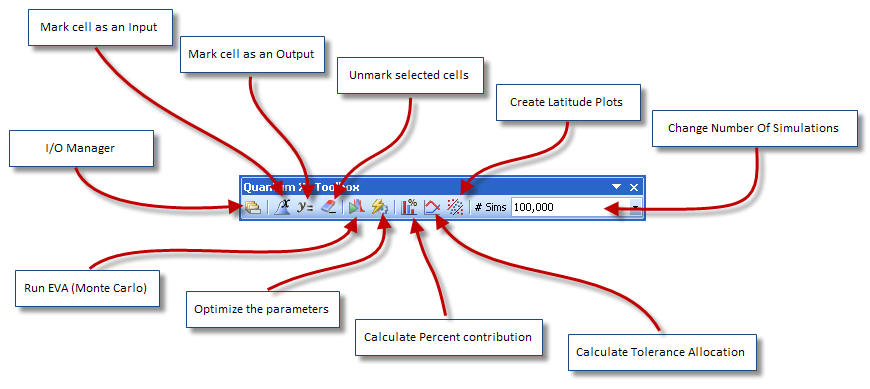
Excel 2000, 2002, and 2003 Shortcut Menu Bar
Excel 2007 Ribbon
