

Quantum XL’s bulk input/output feature allows the rapid creation of models with large numbers of inputs. To demonstrate how to use this feature, we will use Quantum XL to analyze the record 1961 season of Roger Maris.
In 1927, Babe Ruth hit 60 home runs, setting the single season record that would stand for more than three decades. Thirty-four years later, in 1961, Roger Maris surpassed Babe Ruth with 61 home runs. (Billy Crystal’s excellent movie 61* provides a fascinating history of the event.) There are many theories as to how someone who had never hit more than 39 home runs in a single season was able to surpass Babe Ruth. They vary from expansion teams that watered down the pitching to a home run race with teammate Mickey Mantle. While I am confident that Mr. Maris had exceptional capability–and since he played well before performance-enhancing drugs had saturated baseball–an interesting question, and the subject of this article, is …
What are the odds that Roger Maris’ record of 61 home runs in 1961 was not the result of a spike in his performance, “watered down pitching”, or any other assignable cause, but was just the result of random variation?
One way to answer this question is to calculate the probability of Mr. Maris hitting a home run in the preceding season (1960), and then use this information in a simulation of the 1961 season. During the regular season in 1960, Mr. Maris hit 39 home runs in 578 trips to the plate. He also hit 2 more home runs in 32 attempts in the post season. Thus, in 1960 he had a total of 41 home runs in 610 attempts, or a 6.72% probability of hitting a home run during each trip to the plate.
To answer the aforementioned question, we still need one more piece of information: how many times did Roger Maris approach the plate in 1961? The answer is 698 times–he had 120 more at bats than in the year before.
Building the Model
Using this information, we can set up a simple Monte Carlo Simulation using Quantum XL to determine the probability that Maris will meet or beat Babe Ruth’s record of 60 home runs in a single year. In Excel, set up a table that looks like the following ….
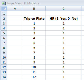
The left column counts the number of trips Maris took to the plate. In the right column, we will show the result of each attempt at bat using the following code.
- Home Run = 1
- Anything other than a home run = 0 (includes strikeout, walk, single, double, etc.)
The table should continue so that it includes one row for each of Roger Maris’ 698 trips to the plate. At the end, we will calculate the total of all of his home runs using Excel’s sum function.
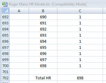
At this point, the total number of home runs is calculated to be 698, which is what would occur if Maris hit a home run on every trip to the plate. Since no one, Roger Maris and Babe Ruth included, could hit a home run on every attempt, we need to modify the sheet so there is a 6.72% chance that the cell will contain a 1. To do this, we can use Quantum XL’s Binary distribution.
Defining the Inputs
- Move your mouse to cell C3.
- Right click and select “Mark Input” (if you do not see the words “Mark Input” when you right click, then you need to start Quantum XL).
- Make the following changes to the Define Input Window:
- Distribution = Binary
- Offset = 0
- Probability of a 1 = .0672
- Press OK.
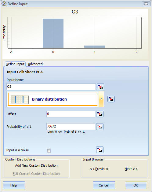
By marking cell C3 as an input with a 6.72% chance of being a 1, we mimic Mr. Maris’ odds of hitting a HR in this particular attempt. Most of the time–specifically 93.28% of the time–the cell will be zero, indicating that the attempt did not result in a HR. However, in a few special occasions (6.72% to be exact), the ball leaves the park and we have a 1.
As the model stands now, only the first attempt has been assigned a 6.72% chance of a home run. We need to make the other 697 cells have the same binary distribution. As you can imagine, this could take a while if we do one cell at a time. To speed this up, we can use Quantum XL’s bulk input/output feature.
Defining an Array of Cells as Inputs Using Quantum XL’s Bulk Input Feature
To mark cells C4 through C700 as inputs, perform the following actions.
- Select cells C4 through C700 (the rest of the column; no need to mark C3 again).
- With the cells selected, right click and select “Mark Input”.
- Make the following changes to the Define Input Window:
- Distribution = Binary
- Offset = 0
- Probability of a 1 = .0672
- Press OK.
Quantum XL will now define all of the cells that were selected as having the same binary distribution. Be patient; this may take 5-10 seconds as there are a lot of cells to mark. When Quantum XL has finished, you should see a small red triangle at the top of each cell. This triangle indicates that the cell has been marked as an input.
Defining the Output using Quantum XL
To collect the proper statistics, we need to tell Quantum XL that cell C702 is the output that we are interested in.
- Go to cell C702.
- Right click and select “Mark Output”.
- Make the following changes to the Define Output Window:
- Output Name = “Total HR”
- LSL = 60
- Click OK.
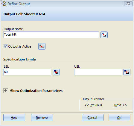
You may find yourself asking the question … “why 60”? The original question was related to the probability of Roger Maris meeting or exceeding Babe Ruth’s record. By setting the LSL to 60, any total number of HRs less than 60 counts as a defect.
Our model is defined; now we can run the simulation. To do this, follow the instructions below based upon your version of Excel.
Excel 2003 and Earlier
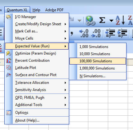
Select “Quantum XL” – “Expected Value (Run)” – “100,000 Simulations”
Excel 2007 or Later
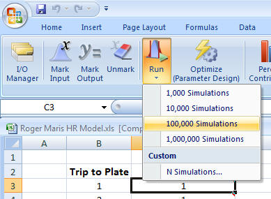
Select “Run” – “100,000 Simulations”
Running 100,000 simulations on a large model like this may take as long as a minute. Quantum XL will display the statistical results when the simulation is complete.
Interpreting the Results
These 100,000 simulations represent the possible outcome of 100,000 hypothetical seasons that Roger Maris could have played. The number of home runs Maris could hit each season would vary based upon a number of random factors, such as the weather, how he feels that day, if the pitcher is throwing spit balls, etc. You could perform the same analysis if you had a coin that when flipped came up heads 6.72% of the time (instead of the presumed 50%). To fully reproduce these results, however, you would need to flip the coin 698 times, keeping track of the number of heads, and then repeat the entire process 99,999 more times.
The histogram below is the graphical result of these 100,000 simulated baseball seasons. The narrow vertical bars represent the number of times an individual season had the specified number of home runs. All the seasons with fewer than 60 home runs are colored red. The seasons with 60 or more home runs are colored blue.
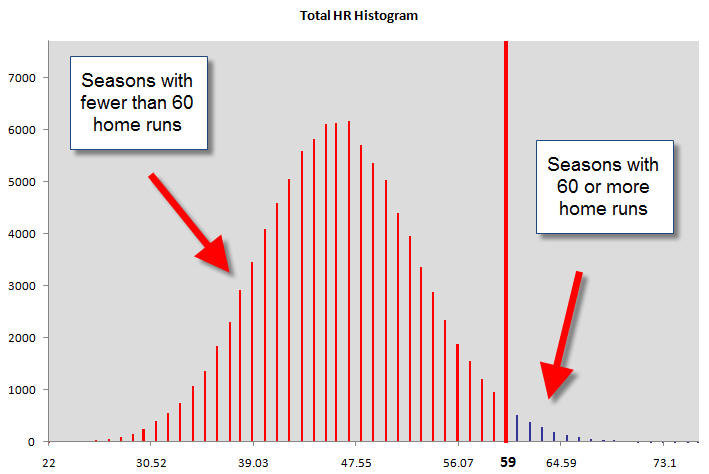
A visual analysis of the histogram shows the small likelihood of having a season with 60 or more home runs. To find out exactly how small, we need to look at the remainder of the analysis. Just below the histogram are the following statistics.
The dpm (defects per million) is the number of seasons with fewer than 60 home runs, scaled to a million. A correct interpretation of the 967,940 dpm is to say that in 96.794% of the seasons, Roger Maris would have hit fewer than 60 home runs. This means that there is a (1-.968)=.032 or 3.2% chance of hitting more than 60 home runs in a season that is due to nothing other than random variation.
While this is not very likely, neither is it a one-in-a-million possibility. We should remember that these are the results of a single season. That Mr. Maris had multiple seasons in which to break the record increases the likelihood that the record would be broken due to random variation.
Other Interesting Notes
My motivation for this article came from The Drunkard’s Walk, How Randomness Rules Our Lives by Leonard Mlodinow, which is without a doubt the best explanation of variation and probability that I have had the pleasure to read. In his book, Mlodinow observes that if you consider all batters of the same capability as Roger Maris in the years after Babe Ruth’s 1927 season, there is a better than 50% probability that one of them would meet or beat the 60 home run record.
A similar analysis could be performed using a simple Binomial calculation, such as the one in SPC XL. However, it wouldn’t be nearly as fun or provide the interesting histogram.
Babe Ruth’s record stood for 34 years before Roger Maris had his famous season. Maris’ record stood for another 38 years, until 1999. Between 1999 and 2001, the 61 HR record was exceeded 6 times–by Sammy Sosa (three times), Mark McGwire (twice), and Barry Bonds (once). This also happens to be the period when baseball has found evidence of performance-enhancing drugs. For an interesting analysis of Barry Bonds and Roger Clemens, see the article Roger Clemens, Barry Bonds, Performance-Enhancing Drugs, and Hypothesis Testing: A Case Study in Baseball and Hypothesis Testing.
For more information about Monte Carlo Simulation in Quantum XL visit the Quantum XL web page.
Brilliant explanation of the illustration in The Drunkard’s Walk, How Randomness Rules Our Lives. I plan to use this in the statistics class I teach.