
Athletes and their purported use of performance-enhancing drugs have dominated the sporting news in the last few months. The controversy seems to be particularly heated in the sport of baseball, with the Mitchell Report naming many famous players. Of particular interest is the accusation by Brian McNamee that Roger Clemens used performance-enhancing drugs to increase his performance. As statistics are readily available in the sport of baseball, I decided to perform a statistical analysis of Mr. Clemens’ performance before and after his alleged use of performance-enhancing drugs.
The field of probability and statistics has formal tests which can be used to determine if an average has changed. These tests are called “Hypothesis Tests” and can be used to help understand whether Roger Clemens’ performance changed before and after the period of alleged drug use. Before I explain the test, let me explain why we need formal Hypothesis tests.
Almost all data has some form of variation. If you don’t believe me, go outside and throw a baseball, football, or whatever kind of ball you prefer as far as you can 10 times. If you measure the distance of each throw, you will find that each of them goes a different distance. Additionally – and here is a key point – one of the 10 throws will be the longest. The problem is that we as humans tend to see this single point and draw conclusions that are not necessarily valid. For example, if the longest throw was one of the latter, then we might say that “we were just getting warmed up”. If the longest was one of the earlier throws, we might say that “our arm got tired at the end”. However, it is possible that the longest throw was simply random. Perhaps there isn’t anything “different” about the throw, it was just another throw in 10 that happened to go the farthest. We don’t tend to think this way. We want to be able to find assignable causes in data so that changes in performance can be explained, and are therefore not random.
What do I mean by an assignable cause? Go outside and throw 10 more balls, but this time throw using your left-hand (or your non-dominant hand). Unless you are different from the vast majority of the people on the planet, there will be a large difference between the distances you threw right-handed vs. left-handed. In this case, the assignable cause is that you changed hands. Changing from your dominant hand changed the distance that the ball went.
In the case of both Roger Clemens and Barry Bonds, the assignable cause would be the purported use of performance-enhancing drugs.
Put more simply, when Mr. Clemens and Mr. Bonds were allegedly taking performance-enhancing drugs, did this make them pitch or bat better? In order to test this theory, we can perform a formal hypothesis test.
Hypothesis Testing
To perform a hypothesis test, we start with two mutually exclusive hypotheses. Here’s an example: when someone is accused of a crime, we put them on trial to determine their innocence or guilt. In this classic case, the two possibilities are the defendant is not guilty (innocent of the crime) or the defendant is guilty. This is classically written as…
H0: Defendant is ← Null Hypothesis
H1: Defendant is Guilty ← Alternate Hypothesis
Unfortunately, our justice systems are not perfect. At times, we let the guilty go free and put the innocent in jail. The conclusion drawn can be different from the truth, and in these cases we have made an error. The table below has all four possibilities. Note that the columns represent the “True State of Nature” and reflect if the person is truly innocent or guilty. The rows represent the conclusion drawn by the judge or jury.
Two of the four possible outcomes are correct. If the truth is they are innocent and the conclusion drawn is innocent, then no error has been made. If the truth is they are guilty and we conclude they are guilty, again no error. However, the other two possibilities result in an error.
A Type I (read “Type one”) error is when the person is truly innocent but the jury finds them guilty. A Type II (read “Type two”) error is when a person is truly guilty but the jury finds him/her innocent. Many people find the distinction between the types of errors as unnecessary at first; perhaps we should just label them both as errors and get on with it. However, the distinction between the two types is extremely important. When we commit a Type I error, we put an innocent person in jail. When we commit a Type II error we let a guilty person go free. Which error is worse? The generally accepted position of society is that a Type I Error or putting an innocent person in jail is far worse than a Type II error or letting a guilty person go free. In fact, in the United States our burden of proof in criminal cases is established as “Beyond reasonable doubt”.
Another way to look at Type I vs. Type II errors is that a Type I error is the probability of overreacting and a Type II error is the probability of under reacting.
In statistics, we want to quantify the probability of a Type I and Type II error. The probability of a Type I Error is α (Greek letter “alpha”) and the probability of a Type II error is β (Greek letter “beta”). Without slipping too far into the world of theoretical statistics and Greek letters, let’s simplify this a bit. What if I said the probability of committing a Type I error was 20%? A more common way to express this would be that we stand a 20% chance of putting an innocent man in jail. Would this meet your requirement for “beyond reasonable doubt”? At 20% we stand a 1 in 5 chance of committing an error. To me, this is not sufficient evidence and so I would not conclude that he/she is guilty.
The formal calculation of the probability of Type I error is critical in the field of probability and statistics. However, the term “Probability of Type I Error” is not reader-friendly. For this reason, for the duration of the article, I will use the phrase “Chances of Getting it Wrong” instead of “Probability of Type I Error”. I think that most people would agree that putting an innocent person in jail is “Getting it Wrong” as well as being easier for us to relate to. To help you get a better understanding of what this means, the table below shows some possible values for getting it wrong.
Chances of Getting it Wrong
(Probability of Type I Error)
| Percentage | Chances of sending an innocent man to jail |
| 20% Chance | 1 in 5 |
| 5% Chance | 1 in 20 |
| 1% Chance | 1 in 100 |
| .01% Chance | 1 in 10,000 |
Roger Clemens Analysis

Unfortunately, court trials do not come with calculations of committing a Type I error. The determination of “reasonable doubt” is much less quantitative. However, statistics does provide numerical values for two different sets of data. Instead of a hypothesis of guilt or innocence, let’s look at Mr. Clemens’ performance in the years that he was accused of using performance-enhancing drugs. Our hypothesis will be….
H0: Mr. Clemens pitched the same before and after 1998
H1: Mr. Clemens pitched different after 1998
I picked the year 1998 since Brian McNamee indicated he started giving Mr. Clemens performance-enhancing drugs in this year. The fact that Brian McNamee gave us the year makes the analysis far easier. It provides a clean break point for before and after. For the analysis of Mr. Clemens, I have included his before years as the years from 1984 to 1997 and the after years as 1998 to 2005. I didn’t include the years 2006 or 2007 as Mr. Clemens didn’t pitch for the full seasons. Thus, for the remainder of this article, Mr. Clemens’ before and after is defined as:
Roger Clemens Alleged Drug Use Periods
Before Alleged Drug Use – 1984 to 1997
After Alleged Drug Use -1998 to 2005
We need a better way to define “pitched better”; luckily, baseball keeps a wealth of statistics on pitchers and batters to give us a quantitative assessment. For pitchers, the most commonly used statistic seems to be ERA (earned run average). The lower the ERA, the better the pitcher. There are other statistics, such as ERA+, WHIP, and win percentage which we will get to in a moment. Mr. Clemens’ ERA before alleged drug use is 3.09 and his ERA after alleged drug use is 3.45. Remembering that a lower ERA is better, his performance after the alleged use is worse than before. The question still remains: did Mr. Clemens’ performance change (for better or worse) after the alleged drug use? Is the difference in ERA from 3.09 to 3.45 due to some assignable cause or is it simply random variation? For this data, the hypothesis test is defined as..
H0: Mr. Clemens’ average ERA was the same before and after
H1: Mr. Clemens’ average ERA was different after alleged drug use
The hypothesis test for this type of data is called a “t-Test”. A t-Test is commonly used to determine if two different data sets have a different average. In our example, we would like to know if the average ERA is different before and after the alleged drug use. The chances of getting it wrong using Mr. Clemens’ ERA data before and after alleged drug use is 35%. (If you are interested in the data behind this article or how to calculate the probability of Type I error click here.) If we conclude that Mr. Clemens’ ERAs changed before and after 1998, we would have a 35% chance of being wrong or roughly a 1 in 3 chance of being incorrect. Most scientists require a level of proof such that the chances of getting it wrong are less than 5% before they will conclude that there is a difference in average. A 35% chance of getting it wrong is too big of a chance and I would conclude that there was no difference in performance. A simple graph called a dot plot can help us compare Mr. Clemens’ performance before and after 1998.
In the graph below, the blue dots represent Mr. Clemens’ ERA in the years before 1998, while the green triangles represent the ERA in the years after 1998. Visually, it does not appear that there is a difference in the average ERA, and the t-Test confirms this.
Barry Bonds Analysis
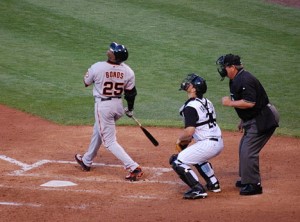
For the analysis of Mr. Bonds, we need to define the years of alleged drug use and pick a suitable statistic. Mr. Bonds has been accused of using performance-enhancing drugs at the end of 1998. Mr. Bonds only participated in 14 games in 2005 due to various factors. This disruption in the normal process provides a good place to break after the alleged drug use; therefore, the before and after periods for Mr. Bonds are defined as…
The key performance metric for batters tends to be their Batting Average (BA). Mr. Bonds’ batting average from 1986 to 1998 is .289, and his average from 1999 to 2004 is .329. Since a larger batting average is better, Mr. Bonds’ average BA did improve in the alleged drug-use years. However, is the difference in his Batting Average due to random variation, or is it large enough to say that he actually improved? The hypothesis test for Mr. Bonds would be…
Barry Bonds Alleged Drug Use Periods
Before Alleged Drug Use – 1986 to 1998
After Alleged Drug Use -1999 to 2004
H0: Mr. Bonds’ average BA was the same before and after
H1: Mr. Bonds’ average BA was different after alleged drug use
I calculated the chances of getting it wrong (probability of a Type I Error) using the available statistics and it came out to 3%. Put another way, if we conclude that Mr. Bonds’ average BA is different during the period of alleged drug use, then we would be wrong only 3 times in 100. As I said before, we typically would like the chance of getting it wrong to be less than 5% to conclude the averages are different. In this case, the chance of getting it wrong is less than 5%, so I would conclude that Mr. Bonds’ average BA did improve after 1998. This difference in average can be seen visually in the dot plot below. The blue dots represent Mr. Bonds’ Batting Average before alleged drug use, and the green triangles represent Mr. Bonds’ BA after alleged drug use. Visually, it appears that the average did increase after 1998. The formal calculation of the Type I error tells us that what we see on the dot plot is in fact a shift in the mean and not just random variation.
Roger Clemens Additional Statistics
While Mr. Clemens’ ERA doesn’t appear to have changed, we can get a clearer picture if we look at statistics other than ERA. Pitchers are also evaluated using the statistic Adjusted ERA+ which adjusts the ERA for ballparks. Since some ballparks favor batters and others pitchers, the ERA+ statistic was created to adjust for this potential bias and normalize pitchers in a more equitable manner. An ERA+ of 100 means that a pitcher performed equal to the average pitcher, with any value over 100 being better than average and any value under 100 being worse than average. Note that for the raw statistic ERA lower is better, and for ERA+ bigger is better. We can also use Walks Plus Hits Per Inning Pitched (WHIP) which is yet another baseball statistic. The lower the WHIP, the better the pitcher.
The table below has the before and after analysis for Mr. Clemens and the associated chances of getting it wrong (Type I error). While Mr. Clemens’ performance was slightly worse in after years, the difference is very small and likely the result of random variation.
Roger Clemens Pitching Statistics Before and After Alleged Drug Use | ||||
| Before (1984-1997) | After (1998-2005) | Chances of Getting it Wrong (Type I Error) | Conclusion | |
| ERA (lower better) | 3.09 | 3.45 | 35% | No change in performance |
| Adjusted ERA+ (higher better) | 152 | 140 | 49% | No change in performance |
| WHIP (lower better) | 1.168 | 1.227 | 35% | No change in performance |
Based upon the analysis of Roger Clemens’ ERA, Adjusted ERA+, and WHIP statistics, there is insufficient statistical evidence to suggest that his average performance changed in the years before and after the alleged use of performance-enhancing drugs.
Barry Bonds Additional Statistics
Similar to pitchers, batters have additional statistics which can be used to measure their performance. For this analysis, I endeavored to use statistics that reflect the individual batter’s performance. For example, I didn’t use RBI (Runs Batted In) as this is dependent on the batters preceding Mr. Bonds. I chose to include On Base Percentage (OBP), Slugging Average (SLG), and everyone’s favorite, the Number of Homeruns. The results for Mr. Bonds are below.
Barry Bonds Hitting Statistics Before and After Alleged Drug Use | ||||
| Before (1986-1998) | After (1998-2004) | Chances of Getting it Wrong (Type I Error) | Conclusion | |
| Batting Average (higher better) | .289 | .329 | 3% | Batting average increased after alleged drug use |
| On Base Percentage (higher better) | .408 | .511 | .3% | Batting average increased after alleged drug use |
| Slugging Average (higher better) | .557 | .755 | .02% | Batting average increased after alleged drug use |
| Home Runs (higher Better) | 31.6 | 48.7 | .4% | Batting average increased after alleged drug use |
The results for Mr. Bonds were quite surprising, as the evidence is overwhelming that the after period was concurrent with increased performance. The most extreme statistic for Mr. Bonds is the Slugging Average (total bases divided by the number of at bats). Batting Average is a simple metric of hits divided by the number of at bats, and doesn’t increase if the hit was a double, triple, or homerun. The Slugging Average includes this information and increases if the batter hits more homeruns and triples than singles and doubles.
For Mr. Bonds, this slugging average before and after alleged drug use increased from .557 to .755. The probability of this occurring randomly is a scant .02% or 2 in 10,000. All four of Mr. Bonds’ batting statistics resulted in a statistically significant increase in performance after the alleged drug use.
Roger Clemens Conclusion
This analysis is limited in scope to Mr. Clemens’ performance in the years prior to and after alleged drug use. I am sure many will argue that his performance should have dropped in his later years due to the natural effects of aging. In fact, Mr. Clemens’ performance did drop; however, the drop was not statistically significant and it appears that his performance before and after alleged drug use was approximately the same.
Is it possible that Mr. Clemens took performance-enhancing drugs? Yes. Assuming for the moment that he did take performance-enhancing drugs, did it increase his performance over previous years? No.
There is little, if any, evidence that Roger Clemens’ performance was increased in the years after the alleged use. Put another way, if Mr. Clemens did take performance-enhancing drugs, he should get his money back.
Barry Bonds Conclusion
The data for Mr. Bonds isn’t nearly so promising. Keep in mind that this article can’t state that Mr. Bonds did or did not take performance-enhancing drugs; it is an analysis of his performance before and after the alleged use. The statistical analysis of the data shows that Mr. Bonds’ hitting performance increased in the years after he allegedly started using performance-enhancing drugs and furthermore, that it is extremely unlikely that this performance increase was random.
Is it possible that Mr. Bonds did not take performance-enhancing drugs? Yes. Assuming for the moment that he did not take the alleged drugs, did his performance still increase? Yes.
There is strong evidence to support that Mr. Bonds’ batting performance increased substantially from 1999 to 2004. If it wasn’t the use of performance-enhancing drugs, then some other assignable cause is likely to be responsible for his performance increase.
Inclusive Dates
Many people will likely disagree on the years that I chose to analyze Mr. Clemens’ and Mr. Bonds’ records. In this section, I will explain my rationale for picking the dates of before and after alleged drug use. The more important concept is that I picked the dates and then afterward performed the statistical analysis. This is distinctly different from looking through the players’ statistics and then picking which years to include.
According to the Mitchell Report, Brian McNamee claims to have given Mr. Clemens steroids in 1998 and human growth hormone (HGH) in 2000 and 2001. I made the assumption that the benefits of these drugs would not be instant on/instant off. In other words, if Mr. Clemens did take HGH in 2000 and 2001 he would continue to see performance gains from this into 2002 and on. Perhaps the benefits of HGH would subside quickly or perhaps they would continue for years. Mr. Clemens didn’t play a full season in the year 2006, and therefore this made a convenient break point. Undoubtedly some will want to analyze the data using a smaller period, perhaps stopping in the year 2002 or 2003. I should note that Mr. Clemens’ career best ERA was in 2005. The inclusion of the 2005 data improves his “after” statistics and yet he still didn’t have a performance increase.
According to the book Game of Shadows by Mark Fainaru-Wada and Lance Williams, Mr. Bonds began steroid use at the end of 1998 with increased frequency and variety until the raid on BALCO in Sept 2003. As the steroid use began in late 1998, I started his after statistics in 1999. Again, assuming that performance gains from the use of these drugs is not instant on/instant off, I chose to include the years after 2003. Mr. Bonds participated in only 14 games in 2005, so this made a convenient break point in the analysis. In the years since 1986, Mr. Bonds had participated in at least 100+ games per season until 2005. Thus, the 2005 season represents a substantial departure from the normal process, and therefore I chose to omit the 2005 and later data.
Statistical Notes
If you are statistically inclined you may have some additional questions. The following section will likely be useful.
- The use of the t-Test assumes normality. The sample sizes were relatively small, making rejection of Normality unlikely. All test of normality failed to reject at the .05 level.
- Additional testing using non-parametric supports the analysis. For example, the p-value using Mood’s Median test on Mr. Bonds’ slugging average results in a p-value of .002.
- For some of the statistics, a Test of Proportions could be used instead of a t-Test. For example, an AB (at bat) can result in a “hit” or not. In this case, each at bat is binomial resulting in the use of the Test of Proportions instead of a t-Test. As the sample size increases the t distribution becomes an excellent approximation of the binomial distribution; however, I did do an analysis using the Test of Proportions for completeness. For example, in the before period Mr. Bonds had 1,917 hits in 6,621 at bats. In the after period he had 813 hits in 2,477 at bats. His proportion of hits increased from 29% to 33% between the two periods. The p-value from the Test of Proportions is .00034 which supports the previous conclusions.
- Use of home runs per season has unequal opportunity. Mr. Bonds did not have the same number of At Bats (AB) in each season. I included Home Runs as a statistic due to the popularity of the statistic only. A better statistic would be home runs per season divided by the number of at bats per season. I do not know if this is an official statistic, but I calculated this for the applicable years. The resulting p-value is .000029 which supports the previous conclusions.
- All analysis was done using a two-sided test (the hypothesis was that the averages were different). A similar analysis could be performed using a single-sided test (the hypothesis would be that the average is greater than or less than). I chose a two-sided, as my entry position was that I wanted to know if there was a difference. For completeness, I did an additional analysis on all tests and they support the previous conclusions.
- The power (Beta or probability of Type II error) is weak due to the limited sample sizes. The fact that we found such significance in Mr. Bonds’ performance with such a small sample size is surprising. However, with more data we might find evidence to suggest that Mr. Clemens’ performance did in fact decrease in the after period.
About the Author
My motivation for writing this article is to provide an interesting example of Hypothesis testing. I am not a baseball fan and frankly wish this would all come to an end so we can get more football news coverage. I have been to one Major League baseball game which was in Chicago in 2006 and happened to coincide with a family vacation. We left after 4 innings. I do not know Roger Clemens or Barry Bonds nor am I associated with either of them in any way.
Pingback: Calculating Type I Probability - SigmaZone
You’re so cool! I do not suppose I’ve truly read a single thing like
this before. So wonderful to discover another person ith original thooughts on this topic.
Seriously.. thanks for starting this up. This site is something that is required on the internet, someone with a bit of originality!
I think this is among the most important information for me.
And i amm glad readijg your article. But should remark on some general things, The site styl
is perfect, the articles is really excellent : D. Good job, cheers
That is very attention-grabbing, You are an excessively professional blogger.
I’ve joined your rss feed and look forward to in the hunt for extra of your magnificent post.
Additionally, I have shared your site in my social networks
Its like you read my mind! You appear to know a lot about
this, like you wrote the book in it or something.
I think that you can do with a few pics to drive the message home a bit,
but other than that, this is wonderful blog. An excellent read.
I’ll definitely be back.
I am actually happy to read this weblog posts which includes lots of
valuable data, thanks for providing such statistics.
Fantastic goods from you, man. I have understand your stuff previous to
and you are just too fantastic. I really like what you’ve acquired here,
really like what you are stating and the way in which you say it.
You make it enjoyable and you still take care of to keep it wise.
I can not wait to read far more from you. This is really a wonderful web site.